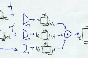
The title is a bit ambitious. More specifically this is
a cheat sheet for some keras merging layers, (untrained) convolutional layers, and activation functions with a comparison of luminance, RGB, HSV, and YCbCR color spaces.
After
experimenting with concatenate layers, I looked at the other merging layers and decided I needed
visual examples of the operations. In these cases, the grayscale/luminance flavors would be the most relevant to machine learning where you're typically working with single-channel feature maps (derived from color images).
I continued with samples of pooling layers and trainable layers with default weights. The latter provided helpful visualizations of activation functions applied to real images.
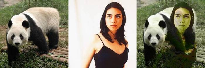
Merging layers
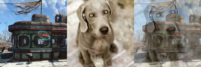
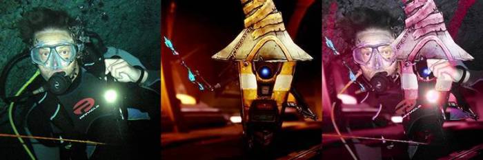
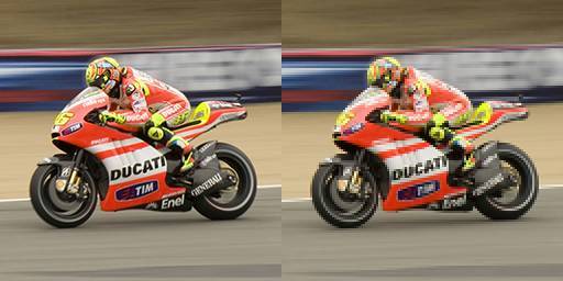
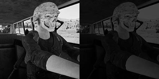
Add
|
|
|
Add layer applied to a single-channel image. |
|
|
|
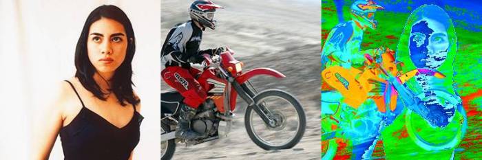
Add in HSV gives you a hue shift. |
|
|
|
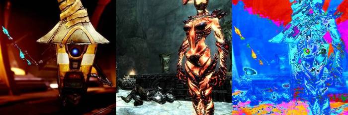
Adding the Cb and Cr channels gives this color space even more of a hue shift. |
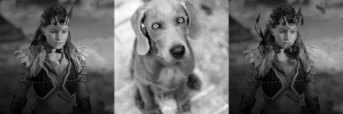
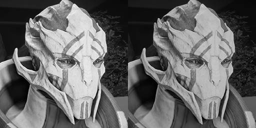
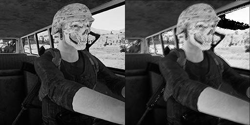
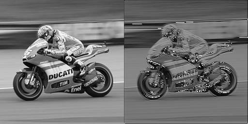
Subtract
|
|
|
Subtraction layer applied to a single-channel image. |
|
|
|
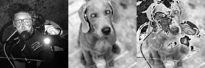
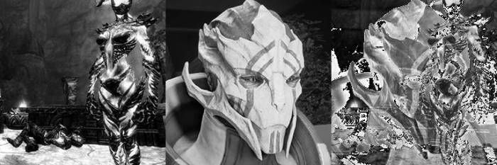
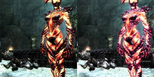
Subtracting YCbCr is pretty deformative. |
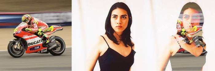
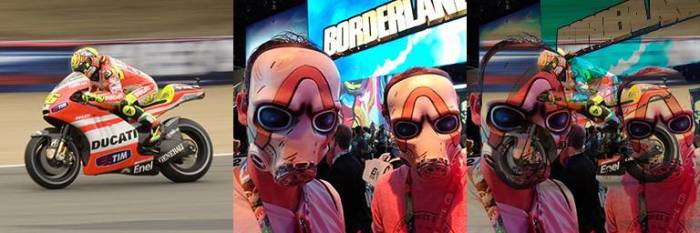
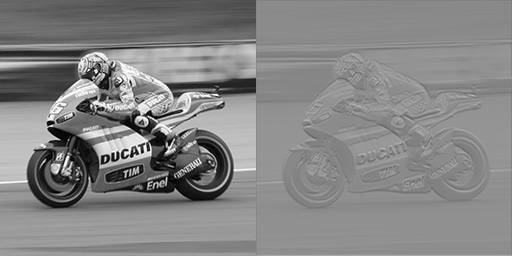
Multiply
|
|
|
Multiply, I guess, makes things darker by the amount of darkness being multiplied (0.0-1.0 values). |
|
|
|
RGB multiply looks similar. |
|
|
|
In HSV, the multiplication is applied less to brightness and more to saturation. |
|
|
|
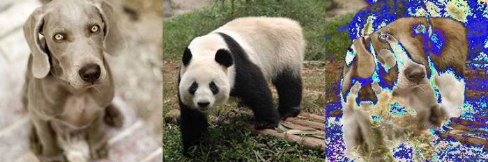
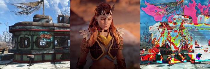
Likewise YCbCr shifts green. |
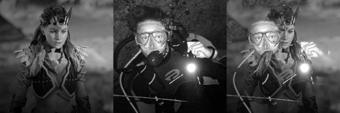
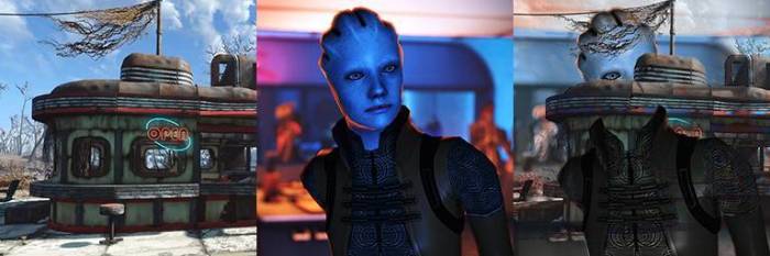
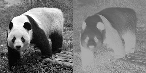
Average
|
|
|
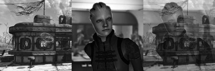
Average in luminance is pretty straightforward. |
|
|
|
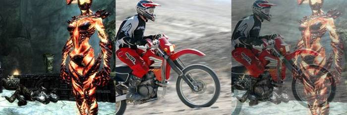
Average in RGB also makes sense. |
|
|
|
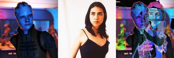
Average in HSV sometimes sees a hue shift. |
|
|
|
Average YCbCr works like RGB. |
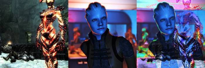
Maximum
|
|
|
Max in monochrome selects the brighter pixel. |
|
|
|
It's not as straightforward in HSV where hue and saturation impact which pixel value is used. |
|
|
|
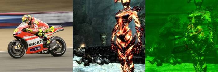
Max for YCbCr likewise biases toward purple (red and blue) pixels. |
Minimum
|
|
|
Minimum, of course, selects the darker pixels. |
|
|
|
In HSV, minimum looks for dark, desaturated pixels with hues happening to be near zero. |
|
|
|
YCbCr looks for dark, greenish pixels. |
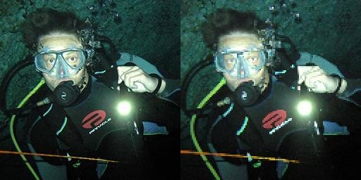
Pooling layers
Most convolutional neural networks use
max pooling to reduce dimensionality. A maxpool layer selects the hottest pixel from a grid (typically 2x2) and uses that value. It's useful for detecting patterns while ignoring pixel-to-pixel noise. Average pooling is another approach that is just as it sounds. I ran 2x2 pooling and then resized the output back up to match the input.
Max pooling
|
|
|
In monochrome images you can see the dark details disappear as pooling selects the brightest pixels. |
|
|
|
RGB behaves similar to luminance. |
|
|
|
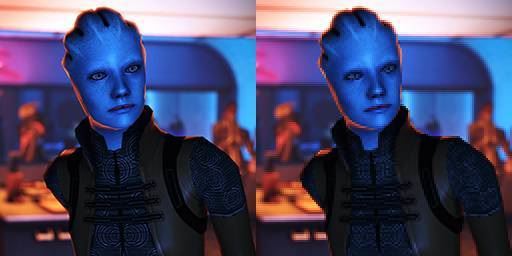
HSV makes the occasional weird selection based on hue and saturation. |
|
|
|
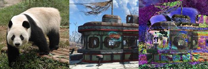
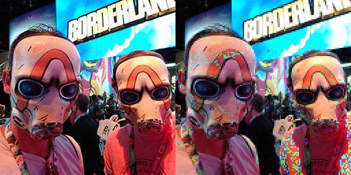
Much like with maximum and minimum from the previous section, maxpooling on YCbCr biases toward the purplest pixel. |
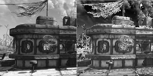
Average pooling
|
|
|
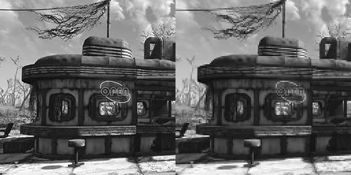
The jaggies (square artifacts) are less obvious in average pooling. |
|
|
|
Edges in RGB look more like antialiasing, flat areas look blurred. |
|
|
|
HSV again shows some occasional hue shift. |
|
|
|
Like with averaging two images, average pooling a single YCbCr image looks just like RGB. |
Dense layers
A couple notes for the trainable layers like Dense:
- I didn't train them, just used glorot_uniform as an initializer. So every run would be different and this wouldn't be reflective of trained layers.
- I stuck to monochrome for simplicity; single-channel input, single layer, single-channel output.
|
|
|
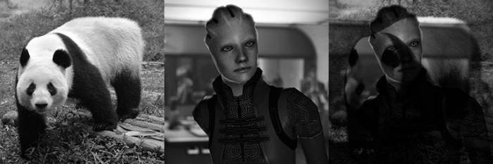
The ReLu looks pretty close to identical. I may not understand the layer, but expected that each output would be fully connected to the inputs. Hmm. |
|
|
|
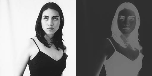
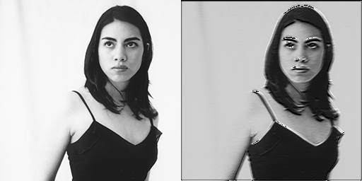
Sigmoid looks like it inverts the input. |
|
|
|
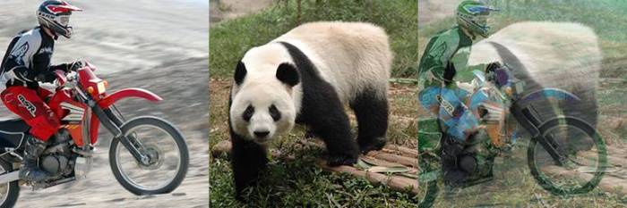
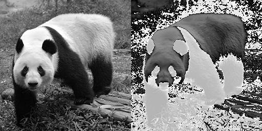
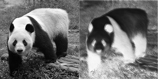
Softplus isn't too fond of the dark parts of the panda. |
|
|
|
Tanh seems to have more or less just darkened the input. |
Not really much to observe here except that the dense nodes seem wired to (or heavily weighted by) their positional input pixel.
Update:
This appears to be the case. To get a fully-connected dense layer you need to flatten before and reshape after. This uses a lot of params though.
Model: "model"
__________________________________________________________________________
Layer (type)                    Output Shape         Param #     Connected
to
==========================================================================
input_1 (InputLayer)            [(None, 32, 32, 1)]  0
__________________________________________________________________________
flatten (Flatten)               (None, 1024)         0           input_1[0]
[0]
__________________________________________________________________________
dense (Dense)                   (None, 1024)         1049600     flatten[0]
[0]
__________________________________________________________________________
input_2 (InputLayer)            [(None, 32, 32, 1)]  0
__________________________________________________________________________
reshape (Reshape)               (None, 32, 32, 1)    0           dense[0]
[0]
==========================================================================
Total params: 1,049,600
Trainable params: 1,049,600
Non-trainable params: 0
__________________________________________________________________________
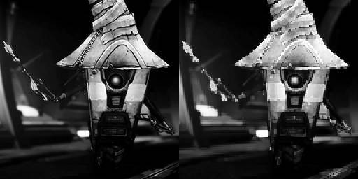
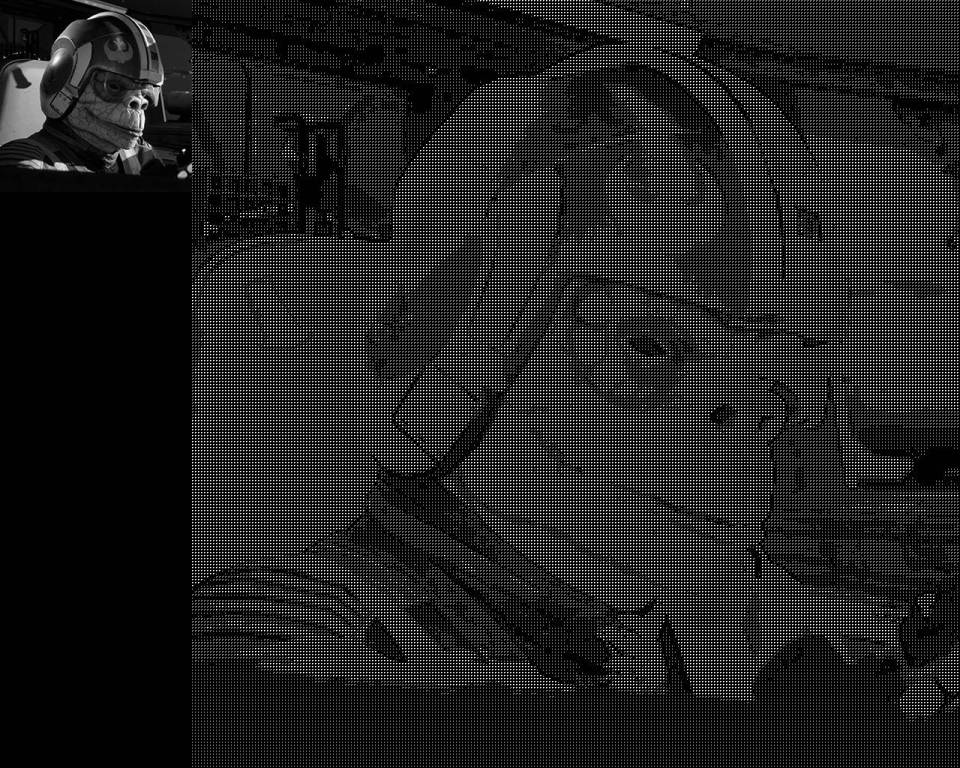
Convolutional layers
As with dense, these runs used kernels with default values.
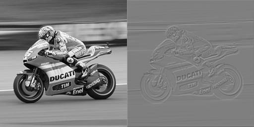
One layer
|
|
|
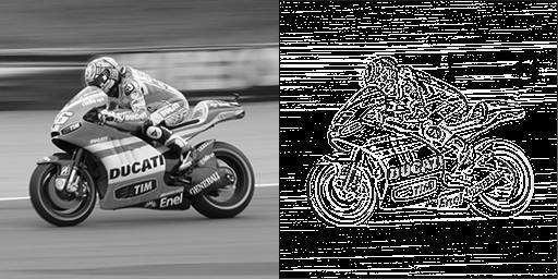
One conv2d layer, kernel size 3, linear activation. |
|
|
|
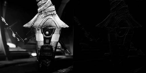
One conv2d layer, kernel size 3, ReLu activation. |
|
|
|
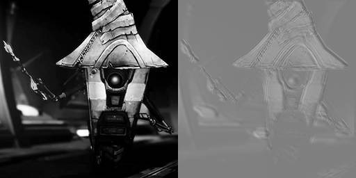
One conv2d layer, kernel size 3, sigmoid activation. |
|
|
|
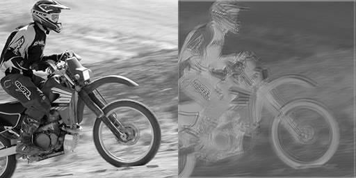
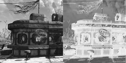
One conv2d layer, kernel size 3, softplus activation. |
|
|
|
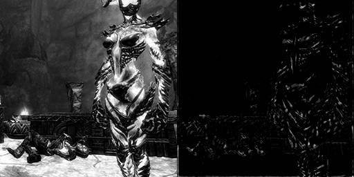
One conv2d layer, kernel size 3, tanh activation. |
This is far more interesting than the dense layers. ReLu seems very good at finding edges/shapes while tanh pushed everything to black and white. What about a larger kernel size?
|
|
|
One conv2d layer, kernel size 7, ReLu activation. |
|
|
|
One conv2d layer, kernel size 7, sigmoid activation. |
|
|
|
One conv2d layer, kernel size 7, softplus activation. |
|
|
|
One conv2d layer, kernel size 7, tanh activation. |
Two layers
|
|
|
Two conv2d layers, kernel size 3, ReLu activation for both. |
|
|
|
Two conv2d layers, kernel size 3, ReLu activation and tanh activation. |
|
|
|
Two conv2d layers, kernel size 3, tanh activation then ReLu activation. |
|
|
|
Two conv2d layers, kernel size 3, tanh activation for both. |
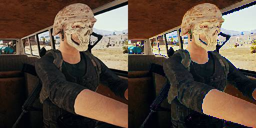
Transpose
Transpose convolution is sometimes used for image generation or upscaling. Using kernel size and striding, this layer (once trained) projects its input onto a (often) larger feature map.
|
|
|
Conv2dTranspose, kernel size 2, strides 2, ReLu activation. |
|
|
|
Conv2dTranspose, kernel size 2, strides 2, sigmoid activation. |
|
|
|
Conv2dTranspose, kernel size 2, strides 4, tanh activation. |
|
|
|
Conv2dTranspose, kernel size 4, strides 2, ReLu activation. |
|
|
|
Conv2dTranspose, kernel size 4, strides 2, tanh activation. |
|
|
|
Conv2dTranspose, kernel size 8, strides 2, ReLu activation. |
|
|
|
Conv2dTranspose, kernel size 8, strides 2, tanh activation. |
Some posts from this site with similar content.
(and some select mainstream web). I haven't personally looked at them or checked them for quality, decency, or sanity. None of these links are promoted, sponsored, or affiliated with this site. For more information, see
.


![[+]](https://www.chrisritchie.org/kilroy/archive/2022/06/leopard.jpg)
![[+]](https://www.chrisritchie.org/kilroy/archive/2015/07/warrior.jpg)
![[+]](https://www.chrisritchie.org/kilroy/archive/2022/05/carousel_ride.jpg)
![[+]](https://www.chrisritchie.org/kilroy/archive/2019/01/viscera_cleanup_mop.jpg)
![[+]](https://www.chrisritchie.org/kilroy/archive/2022/05/elden_ring_jarburg.jpg)
![[+]](https://www.chrisritchie.org/kilroy/archive/2015/02/far_cry_view_00.jpg)
![[+]](https://www.chrisritchie.org/kilroy/archive/2022/04/volleyball_bump.jpg)
![[+]](https://www.chrisritchie.org/kilroy/archive/2017/05/dying_light_stadium.jpg)
![[+]](https://www.chrisritchie.org/kilroy/archive/2022/05/elden_ring_flamethrower.jpg)
![[+]](https://www.chrisritchie.org/kilroy/archive/2016/04/division_helo_00.jpg)
![[+]](https://www.chrisritchie.org/kilroy/archive/2022/04/zinsco_panel.jpg)
![[+]](https://www.chrisritchie.org/kilroy/archive/2015/11/deezer.jpg)
![[+]](https://www.chrisritchie.org/kilroy/archive/2022/04/breaker_test.jpg)
![[+]](https://www.chrisritchie.org/kilroy/archive/2016/08/witches_lair.jpg)